Preliminary Analysis
Jaewon Royce Choi
6/15/2020
Preliminary statistical analysis of relationships between the variables.
library(tidyverse)
library(ggplot2)
library(gridExtra)

#### Read in the dataset ####

tx_bb_entrepreneur_merged <- read_csv("https://raw.githubusercontent.com/jwroycechoi/broadband-entrepreneurship/master/Datasets/Broadband-Entrepreneurship-TX-merged_v2.csv")

str(tx_bb_entrepreneur_merged)
Correlation Matrix for Preliminary Set of Variables
Basic correlation matrix with some preliminary variables.
- IRR2010: Rural index (larger = rural)
- proprietors_2017: # of sole proprietors in TX
- pct_proprietors_employment_2017: % of sole proprietors in total employment
- pct_broadband_FCC: FCC broadband availability in % (2017)
- pct_broadband_MS: MS broadband availability in % (2019)
- venturedensitydec19: Venture density by GoDaddy
- highlyactive_vddec19: Highly active venture density by GoDaddy
- prosperityindex2016: Prosperity index
- frac_BB.dec: % of M-Lab testers with over 25mbps of DL speed & 3mbps of UL
#### Correlation between variabes ####

## Basic Correlation Table ##

tx_bb_entrepreneur_merged %>%
  select(IRR2010, proprietors_2017, pct_proprietors_employment_2017, pct_broadband_FCC, pct_broadband_MS,
         venturedensitydec19, highlyactive_vddec19, prosperityindex2016, frac_BB.dec) %>%
cor(method = "pearson", use = "complete.obs") %>% knitr::kable(format = "markdown", digits = 3)| IRR2010 | proprietors_2017 | pct_proprietors_employment_2017 | pct_broadband_FCC | pct_broadband_MS | venturedensitydec19 | highlyactive_vddec19 | prosperityindex2016 | frac_BB.dec | |
|---|---|---|---|---|---|---|---|---|---|
| IRR2010 | 1.000 | -0.696 | 0.471 | -0.440 | -0.739 | -0.443 | -0.378 | -0.413 | -0.519 |
| proprietors_2017 | -0.696 | 1.000 | -0.226 | 0.227 | 0.465 | 0.363 | 0.315 | 0.281 | 0.278 |
| pct_proprietors_employment_2017 | 0.471 | -0.226 | 1.000 | -0.318 | -0.361 | 0.053 | 0.194 | -0.001 | -0.234 |
| pct_broadband_FCC | -0.440 | 0.227 | -0.318 | 1.000 | 0.535 | 0.183 | 0.080 | 0.266 | 0.453 |
| pct_broadband_MS | -0.739 | 0.465 | -0.361 | 0.535 | 1.000 | 0.541 | 0.482 | 0.610 | 0.687 |
| venturedensitydec19 | -0.443 | 0.363 | 0.053 | 0.183 | 0.541 | 1.000 | 0.790 | 0.533 | 0.270 |
| highlyactive_vddec19 | -0.378 | 0.315 | 0.194 | 0.080 | 0.482 | 0.790 | 1.000 | 0.540 | 0.242 |
| prosperityindex2016 | -0.413 | 0.281 | -0.001 | 0.266 | 0.610 | 0.533 | 0.540 | 1.000 | 0.293 |
| frac_BB.dec | -0.519 | 0.278 | -0.234 | 0.453 | 0.687 | 0.270 | 0.242 | 0.293 | 1.000 |
Correlation Matrix with more Information
A correlation matrix with more in-depth information using the chart.Correlation() function in package PerformanceAnalytics.
#install.packages("PerformanceAnalytics")

tx_bb_entrepreneur_merged %>%
  select(IRR2010, proprietors_2017, pct_proprietors_employment_2017, pct_broadband_FCC, pct_broadband_MS,
         venturedensitydec19, highlyactive_vddec19, prosperityindex2016, frac_BB.dec) %>%
  PerformanceAnalytics::chart.Correlation(histogram = T)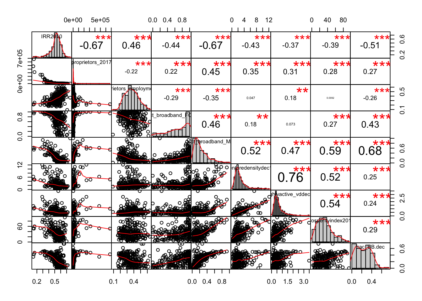
Preliminary Exploration of Relationships further with Regressions
Few models to examine relationships between entrepreneurship and broadband. In general, I take the entrepreneurship measures as the dependent variable and others as the independent. Following the ASU white paper analysis, venture density is explored as a measure of entrepreneurial activities online. Sole proprietors share in total employment is taken into IV as it represents general small-mid sized business activities, but not all of them are active online as reflected in the venture density factor.
#### Exploring the relationships further with regressions ####

## DV: Venture Density as Entrepreneurship Index
## IV: Rural index, Proprietors share in employment, Broadband (FCC), Broadband (MS), Broadband (M-Lab), Broadband Subscription
#install.packages("stargazer")
library(stargazer)

prem_model <- lm(venturedensitydec19 ~ IRR2010 + pct_proprietors_employment_2017 + pct_broadband_FCC + pct_broadband_MS + frac_BB.dec + pctbbfrac_ASU, data = tx_bb_entrepreneur_merged)

## DV: Highly active venture density

prem_model2 <- lm(highlyactive_vddec19 ~ IRR2010 + pct_proprietors_employment_2017 + pct_broadband_FCC + pct_broadband_MS + frac_BB.dec + pctbbfrac_ASU, data = tx_bb_entrepreneur_merged)

## DV: Proprietor's share in employment as an indicator of entrepreneurship

prem_model3 <- lm(pct_proprietors_employment_2017 ~ IRR2010 + pct_broadband_FCC + pct_broadband_MS + frac_BB.dec + pctbbfrac_ASU, data = tx_bb_entrepreneur_merged)| Dependent variable: | |||
| Venture Density | Highly Active VD | Proprietors Share | |
| (1) | (2) | (3) | |
| Rurality Index (2010) | -4.761** | -1.319*** | 0.553*** |
| (1.877) | (0.423) | (0.100) | |
| Proprietors Share (2017) | 5.727*** | 2.001*** | |
| (1.183) | (0.267) | ||
| Broadband (FCC) | -0.698 | -0.293*** | -0.059** |
| (0.456) | (0.103) | (0.026) | |
| Broadband (MS) | 5.998*** | 1.494*** | -0.077 |
| (1.113) | (0.251) | (0.063) | |
| Broadband (M-Lab) | -2.579*** | -0.489** | 0.037 |
| (0.924) | (0.208) | (0.053) | |
| Broadband Subscription (ACS) | 5.608*** | 0.758** | 0.297*** |
| (1.500) | (0.338) | (0.083) | |
| Constant | -0.874 | 0.068 | -0.089 |
| (1.505) | (0.339) | (0.086) | |
| Observations | 226 | 226 | 226 |
| R2 | 0.451 | 0.466 | 0.281 |
| Adjusted R2 | 0.436 | 0.452 | 0.265 |
| F Statistic | 30.028*** (df = 6; 219) | 31.881*** (df = 6; 219) | 17.205*** (df = 5; 220) |
| Note: | p<0.1; p<0.05; p<0.01 | ||
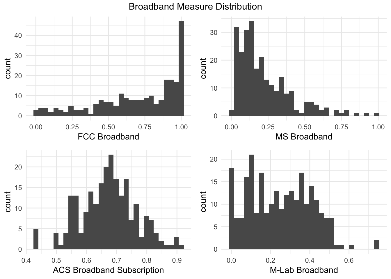
Comaparing Different Broadband Measures
Preliminary explorations reveal interesting discrepancies between different measures of broadband. Here I will explore how these measures paint different pictures of broadband of Texas.
#### Comparing Broadband Measures in the Dataset ####

## Broadband measures
## pct_broadband_FCC: FCC's broadband availability (reported by the service providers)
## pct_broadband_MS: MS's broadband availability (reported by the MS software service users)
## frac_BB.dec: Broadband speed users' share based on M-Lab data (reported by the M-Lab test respondents)
## pctbbfrac_ASU: ASU team's measure derived from the ACS survey estimates (based on reported BB subscription info from respondents)

## Summarize some key statistics of all these broadband variables

# Some basic statistics
tx_bb_entrepreneur_merged %>%
  select(c("pct_broadband_FCC", "pct_broadband_MS", "frac_BB.dec", "pctbbfrac_ASU")) %>%
psych::describe() %>% knitr::kable(digits = 3)| vars | n | mean | sd | median | trimmed | mad | min | max | range | skew | kurtosis | se | |
|---|---|---|---|---|---|---|---|---|---|---|---|---|---|
| pct_broadband_FCC | 1 | 248 | 0.702 | 0.287 | 0.775 | 0.738 | 0.289 | 0.000 | 1.000 | 1.000 | -0.821 | -0.391 | 0.018 |
| pct_broadband_MS | 2 | 254 | 0.223 | 0.185 | 0.165 | 0.194 | 0.141 | 0.010 | 1.000 | 0.990 | 1.484 | 2.232 | 0.012 |
| frac_BB.dec | 3 | 249 | 0.247 | 0.160 | 0.241 | 0.243 | 0.200 | 0.000 | 0.741 | 0.741 | 0.258 | -0.654 | 0.010 |
| pctbbfrac_ASU | 4 | 232 | 0.672 | 0.093 | 0.675 | 0.672 | 0.086 | 0.426 | 0.908 | 0.482 | -0.048 | 0.023 | 0.006 |
# Who are the counties with minimum BB?

# According to FCC BB data
tx_bb_entrepreneur_merged[which(tx_bb_entrepreneur_merged$pct_broadband_FCC == min(tx_bb_entrepreneur_merged$pct_broadband_FCC, na.rm = T)),]$county
## [1] "Llano County" "Upton County"# According to MS BB data
tx_bb_entrepreneur_merged[which(tx_bb_entrepreneur_merged$pct_broadband_MS == min(tx_bb_entrepreneur_merged$pct_broadband_MS, na.rm = T)),]$county## [1] "Borden County" "Kenedy County"# According to M-Lab BB data
tx_bb_entrepreneur_merged[which(tx_bb_entrepreneur_merged$frac_BB.dec == min(tx_bb_entrepreneur_merged$frac_BB.dec, na.rm = T)),]$county## [1] "Briscoe County" "Castro County" "Cochran County"
## [4] "Crane County" "Culberson County" "Delta County"
## [7] "Donley County" "Hartley County" "Jim Hogg County"
## [10] "Kinney County" "McMullen County" "Mitchell County"
## [13] "Newton County" "Refugio County" "Roberts County"
## [16] "San Augustine County" "Sherman County" "Sterling County"# According to ACS BB data
tx_bb_entrepreneur_merged[which(tx_bb_entrepreneur_merged$pctbbfrac_ASU == min(tx_bb_entrepreneur_merged$pctbbfrac_ASU, na.rm = T)),]$county## [1] "Terrell County"# Who are the counties with maximum BB?
# According to FCC BB data
tx_bb_entrepreneur_merged[which(tx_bb_entrepreneur_merged$pct_broadband_FCC == max(tx_bb_entrepreneur_merged$pct_broadband_FCC, na.rm = T)),]$county## [1] "Aransas County" "Bastrop County" "Baylor County"
## [4] "Bee County" "Bexar County" "Bosque County"
## [7] "Brown County" "Caldwell County" "Cameron County"
## [10] "Dallas County" "Denton County" "DeWitt County"
## [13] "Ellis County" "Erath County" "Gonzales County"
## [16] "Grayson County" "Guadalupe County" "Hill County"
## [19] "Hood County" "Johnson County" "Karnes County"
## [22] "Kleberg County" "Knox County" "Lampasas County"
## [25] "Live Oak County" "McLennan County" "McMullen County"
## [28] "Nueces County" "Palo Pinto County" "Parker County"
## [31] "San Patricio County" "Somervell County" "Tarrant County"
## [34] "Travis County" "Willacy County" "Wilson County"
## [37] "Wise County"# According to MS BB data
tx_bb_entrepreneur_merged[which(tx_bb_entrepreneur_merged$pct_broadband_MS == max(tx_bb_entrepreneur_merged$pct_broadband_MS, na.rm = T)),]$county## [1] "Loving County"# According to M-Lab BB data
tx_bb_entrepreneur_merged[which(tx_bb_entrepreneur_merged$frac_BB.dec == max(tx_bb_entrepreneur_merged$frac_BB.dec, na.rm = T)),]$county## [1] "Motley County" "Stonewall County"# According to ACS BB data
tx_bb_entrepreneur_merged[which(tx_bb_entrepreneur_merged$pctbbfrac_ASU == max(tx_bb_entrepreneur_merged$pctbbfrac_ASU, na.rm = T)),]$county## [1] "Fort Bend County"## Take a look at the frequency distribution of each BB measures
grid.arrange(
ggplot(tx_bb_entrepreneur_merged, aes(x = pct_broadband_FCC)) + geom_histogram() + theme_minimal() + xlab("FCC Broadband"),
ggplot(tx_bb_entrepreneur_merged, aes(x = pct_broadband_MS)) + geom_histogram() + theme_minimal() + xlab("MS Broadband"),
ggplot(tx_bb_entrepreneur_merged, aes(x = pctbbfrac_ASU)) + geom_histogram() + theme_minimal() + xlab("ACS Broadband Subscription"),
ggplot(tx_bb_entrepreneur_merged, aes(x = frac_BB.dec)) + geom_histogram() + theme_minimal() + xlab("M-Lab Broadband"),
nrow = 2, ncol = 2, top = "Broadband Measure Distribution"
)
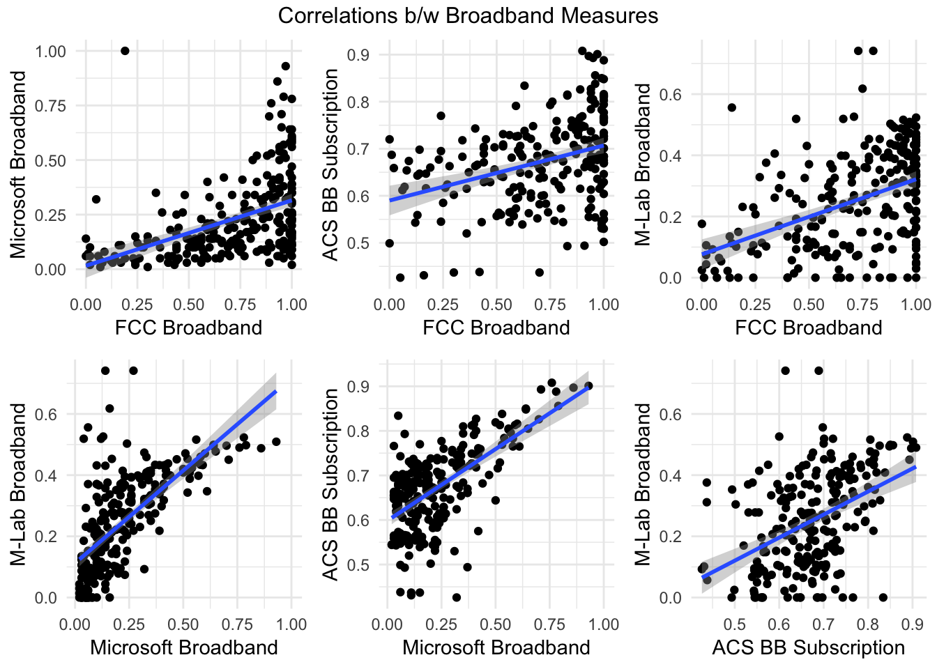
## Plotting relationships between BB measures

grid.arrange(
  ggplot(tx_bb_entrepreneur_merged, aes(x = pct_broadband_FCC, y = pct_broadband_MS)) + geom_point() + geom_smooth(method = "lm") + theme_minimal() + ylab("Microsoft Broadband") + xlab("FCC Broadband"),
  ggplot(tx_bb_entrepreneur_merged, aes(x = pct_broadband_FCC, y = pctbbfrac_ASU)) + geom_point() + geom_smooth(method = "lm") + ylab("ACS BB Subscription") + xlab("FCC Broadband") + theme_minimal(),
  ggplot(tx_bb_entrepreneur_merged, aes(x = pct_broadband_FCC, y = frac_BB.dec)) + geom_point() + geom_smooth(method = "lm") + theme_minimal() + ylab("M-Lab Broadband") + xlab("FCC Broadband"),
  ggplot(tx_bb_entrepreneur_merged, aes(x = pct_broadband_MS, y = frac_BB.dec)) + geom_point() + geom_smooth(method = "lm") + theme_minimal() + ylab("M-Lab Broadband") + xlab("Microsoft Broadband"),
  ggplot(tx_bb_entrepreneur_merged, aes(x = pct_broadband_MS, y = pctbbfrac_ASU)) + geom_point() + geom_smooth(method = "lm") + ylab("ACS BB Subscription") + xlab("Microsoft Broadband") + theme_minimal(),
  ggplot(tx_bb_entrepreneur_merged, aes(x = pctbbfrac_ASU, y = frac_BB.dec)) + geom_point() + geom_smooth(method = "lm") + theme_minimal() + ylab("M-Lab Broadband") + xlab("ACS BB Subscription"),
  nrow = 2, ncol = 3, top = "Correlations b/w Broadband Measures"
)
Copyright © 2020 Jaewon Royce Choi, TIPI. All rights reserved.